
The most reliable safety stock formula for most SKUs is the statistical one that accounts for both demand and lead-time variability: SS = Z × √(LT × σD² + D² × σL²). It beats simpler rules because it captures the real source of stockouts, which is variability compounding across the replenishment cycle, not just average demand. Use it for your A and B items. Save the cruder methods for C items where the data doesn’t justify the extra math.
Here’s the quick reference before you build anything in a spreadsheet:
- Full statistical formula: SS = Z × √(E(L) × σD² + E(D)² × σL²) — use when you have reliable demand and lead-time history.
- Simplified demand-only formula: SS = Z × σD × √L — use when lead time is essentially fixed.
- Max-min formula: SS = (Max Daily Demand × Max Lead Time) − (Avg Daily Demand × Avg Lead Time) — use for thin data or when you want a conservative, easy-to-explain number.
- Fixed-days-of-supply: SS = Avg Daily Demand × Buffer Days — use for low-value, low-risk C items where precision isn’t worth the effort.
- EOQ-linked buffer: safety stock sized as a percentage of your economic order quantity, useful when order cycles are long and reviews are periodic.
Most of what you’ll need to source these inputs already sits inside your ERP: sales history for demand variance, purchase order receipt logs for lead-time variance, and a service-level target your leadership has already implicitly chosen through fill-rate expectations. Mapping a service level to a Z-score is a five-minute lookup once you know the table (more on that below). Getting the inputs right, and knowing when the statistical formula’s assumptions don’t hold, is where most teams either overspend on inventory or under-protect their bestsellers. If your team is rolling this out across hundreds or thousands of SKUs and the internal bandwidth isn’t there, firms like 3plcowboy work directly on this kind of policy design and ERP parameterization.
| Point | Details |
|---|---|
| Default formula | Use the combined statistical formula for A/B SKUs with usable demand and lead-time history. |
| Simplify when justified | Drop to Z × σD × √L only when lead time barely varies. |
| Protect low-data SKUs | Use max-min or fixed-days buffers for C items or new products without history. |
| Service level drives cost | Moving from 95% to 99% service level can raise required safety stock by roughly 40% in typical examples, so reserve high targets for critical items. |

Key Takeaways
The statistical safety stock formula, SS = Z × √(E(L) × σD² + E(D)² × σL²), is the practical default for A and B SKUs, while max-min and fixed-days rules serve low-data C items best.
| Point | Details |
|---|---|
| Default to the statistical formula | Use it for A and B SKUs whenever you have 12+ months of clean demand and lead-time data. |
| Reserve simpler methods for C items | Max-min or fixed-days buffers work fine for low-value, low-data SKUs. |
| ROP depends directly on SS | Reorder point equals expected lead-time demand plus your calculated safety stock. |
| Watch the service-level cost curve | Pushing service level from 95% to 99% can raise safety stock by roughly 40%, so reserve that tier for critical SKUs only. |
| Monitor fill rate after rollout | Track fill rate and inventory days of supply weekly during any pilot, and bring in advisory support like 3plcowboy if a catalog-wide rollout outpaces internal capacity. |
Table of Contents
- What Is Safety Stock and Why Reorder Point Depends on It
- The Terms You Need to Measure Consistently
- Which Method Fits Your Situation
- The Formulas, Explained Term by Term
- A Worked Example You Can Copy Into Excel
- Getting σD and σL Right From Your Own Data
- Matching the Method to Your SKU Tier
- Where These Formulas Break Down
- When to Move Beyond the Standard Formula
- How Safety Stock Plugs Into Your Reorder Point and Ordering Policy
- A Repeatable Checklist for Calculating and Maintaining Safety Stock
- What I’ve Learned Watching Safety Stock Policies Succeed and Fail
- Getting Help Implementing a Safety Stock Policy Across Your Catalog
- Sources
What Is Safety Stock and Why Reorder Point Depends on It
Safety stock is the extra inventory you hold above expected lead-time demand specifically to absorb the unpredictable part of your supply chain: demand spikes you didn’t forecast, and supplier delays that push your lead time past its average. It is not the same as cycle stock, which is the inventory you order and burn through in the normal replenishment rhythm. Cycle stock covers what you expect to sell. Safety stock covers what you don’t expect but should still plan for.
This distinction matters because it determines your reorder point. The standard formula is:
ROP = Expected Lead-Time Demand + Safety Stock
If you sell 50 units a day and your supplier takes 10 days to deliver, expected lead-time demand is 500 units. Without safety stock, you’d place a reorder the moment inventory hits exactly 500, and any demand spike or shipping delay during those 10 days puts you at zero. Add a safety stock buffer of 150 units, and your ROP becomes 650. Now a bad week doesn’t turn into a stockout.
Here’s a quick way to see the split: if your average monthly demand is 1,500 units, and your on-hand inventory sits at 2,000 right after a replenishment, roughly 1,500 of that is cycle stock earmarked for expected sales, and the remaining 500 is your safety buffer sitting quietly in the background.
Why does this matter beyond avoiding empty shelves? Three reasons carry real financial weight:
- Service level targets are a business decision, not a warehouse decision. A 98% service level on your top revenue SKU protects sales; the same target on a slow-moving accessory just ties up cash.
- Working capital gets consumed by safety stock sitting idle. Every unit of buffer inventory is money not available for other investments.
- ERP reorder triggers only work correctly if the ROP field reflects a defensible safety stock number, not a guess someone typed in three years ago and never revisited.
Pro Tip: Pull up your ERP’s current ROP values for your top 20 SKUs by revenue and check when they were last recalculated. If it’s been more than a year, treat that as a red flag regardless of how well things have been going.
The Terms You Need to Measure Consistently
Every safety stock calculation depends on a handful of inputs, and if you get the units wrong, the formula produces a number that looks precise but is functionally useless. Here’s what each term means and where to actually find it.
- E(D) — average demand per period (daily or weekly), pulled from sales history in your ERP.
- σD — standard deviation of demand, measuring how much daily or weekly sales swing around that average.
- E(L) — average lead time, the time between placing a purchase order and receiving usable stock.
- σL — standard deviation of lead time, capturing how unreliable your supplier’s delivery timing actually is.
- Z — the service-level z-score, a statistical multiplier tied to how much protection against stockouts you want.
- Forecast error — the gap between what you predicted and what actually happened, often used as a proxy for σD when demand history is thin.
The single biggest technical mistake teams make here is mixing time units. If your demand is measured daily but your lead time is measured in weeks, the formula will run and spit out a number, but that number will be wrong by a wide margin. Pick one time unit, usually daily, and convert everything into it before you touch the formula.
| Term | What it measures | Where to source it |
|---|---|---|
| E(D) | Average demand per day | ERP sales history, ideally 12+ months |
| σD | Demand variability | Standard deviation function on daily sales data |
| E(L) | Average supplier lead time | PO issue date to goods-receipt date in ERP/WMS |
| σL | Lead-time variability | Standard deviation of the same PO receipt timestamps |
| Z | Desired service level | Standard normal distribution table or Excel’s NORM.S.INV |
A few pitfalls show up constantly. Seasonality inflates σD if you calculate it across a full year without adjusting for peak months, which overstates your buffer needs in the off-season and understates them right before your busy period. Promotions do the same thing in reverse; a single spike from a flash sale can distort your standard deviation for months if you don’t isolate it. And intermittent demand, common in spare parts or long-tail SKUs, breaks the standard deviation calculation entirely because too many periods show zero sales. For those SKUs, a moving-window calculation or a Croston-style approach handles the gaps far better than a raw standard deviation.
Which Method Fits Your Situation
Not every SKU deserves the same level of statistical rigor, and treating them all identically is one of the more expensive mistakes a planning team can make according to guidance from the Institute for Supply Management. Here’s a quick rundown of the main approaches and where each one earns its keep.
- Full statistical formula — best when you have solid demand and lead-time history and want the most defensible number. Higher computational effort, but it’s the gold standard for A and B items.
- Simplified demand-only formula — a good middle ground when your supplier is reliably on time and lead-time variance is close to zero, letting you skip a variable without much accuracy loss.
- Max-min method — the conservative choice for new SKUs or thin sales history, since it uses worst observed values rather than statistical estimates.
- Fixed-days buffer — the simplest rule of all, just holding a set number of days of average demand; fast to implement, but it ignores actual variability entirely.
- EOQ-linked approaches — useful when your order sizing is already driven by economic order quantity logic and you want the safety buffer to scale with order cycle length.
- Simulation (Monte Carlo) — reserved for high-value, high-risk SKUs where demand doesn’t follow a normal distribution and a closed-form formula would mislead you.
The trade-off across all six is roughly linear: more statistical sophistication buys you tighter, more capital-efficient inventory, but it demands cleaner data and more setup time. A rough default by SKU class: statistical formula for A items, statistical or simplified for B items, and max-min or fixed-days for C items where the labor of building a rigorous model outweighs the inventory dollars at stake.
The Formulas, Explained Term by Term
The combined-variance statistical formula is the one worth memorizing, because it’s the only version that accounts for the fact that both your demand and your supplier’s timing can go sideways at the same time. Written out:
SS = Z × √( E(L) × σD² + E(D)² × σL² )
Each term does specific work. Z is your service-level multiplier. E(L) is average lead time, multiplying against demand variance because a longer lead time gives demand more opportunity to swing away from its average. σD² is demand variance itself. E(D)² is squared average demand, multiplying against lead-time variance because a late shipment matters far more when your average daily demand is high than when it’s a trickle. σL² is lead-time variance, capturing how unpredictable your supplier actually is. This full form is the standard reference used across most supply chain calculators precisely because it doesn’t assume your supplier is perfectly on time.
When lead-time variability is negligible, meaning your supplier hits the same delivery window almost every time, the formula collapses to a simpler version:
SS = Z × σD × √L
The square root of lead time isn’t arbitrary. It comes from how variance accumulates across independent time periods: if each day’s demand variance is independent of the next, total variance over a multi-day lead time adds up, and standard deviation, being the square root of variance, scales with the square root of the number of days rather than the number itself.
The max-min method skips the statistics entirely:
SS = (Max Daily Demand × Max Lead Time) − (Avg Daily Demand × Avg Lead Time)
This produces a genuinely conservative number by comparing your absolute worst-case scenario against your average case. Practical calculators built for procurement teams often present this alongside the statistical formula precisely because it requires no distribution assumptions at all, just your highest observed values.
Every one of these formulas assumes demand and lead time are statistically independent of each other, that your demand roughly follows a normal distribution, and that historical variability is a fair predictor of future variability. When any of those three assumptions breaks, and they break more often than most planning teams assume, the formula still runs and still produces a number. That number just stops meaning what you think it means.
Getting Z in Excel is a one-line formula: =NORM.S.INV(0.95) returns roughly 1.645 for a 95% service level, and =NORM.S.INV(0.99) returns roughly 2.326 for 99%. No lookup table needed once you know the syntax.
Statistic in focus: raising your service-level target from 95% to 99% can push required safety stock up by roughly 40% in typical examples, which is exactly why 99% targets belong on your top-tier SKUs only, not blanket-applied across your catalog.
A Worked Example You Can Copy Into Excel
Let’s run real numbers through both approaches so you can see how they diverge.
Example A: Full statistical formula with demand and lead-time variance
Say you’re planning safety stock for a mid-tier SKU with the following inputs: average daily demand (E(D)) of 40 units, demand standard deviation (σD) of 12 units, average lead time (E(L)) of 7 days, lead-time standard deviation (σL) of 2 days, and a target service level of 95% (Z = 1.645).
| Input | Value | Excel formula |
|---|---|---|
| E(D) | 40 | =AVERAGE(daily sales range) |
| σD | 12 | =STDEV.S(daily sales range) |
| E(L) | 7 | =AVERAGE(PO lead-time range) |
| σL | 2 | =STDEV.S(PO lead-time range) |
| Z (95%) | 1.645 | =NORM.S.INV(0.95) |
| Term 1: LT × σD² | 7 × 12² = 1,008 | =E(L)*σD^2 |
| Term 2: E(D)² × σL² | 40² × 4 = 6,400 | =E(D)^2*σL^2 |
| Sum under root | 1,008 + 6,400 | =Term1+Term2 |
| √Sum | √(1,008 + 6,400) | =SQRT(1,008 + 6,400) |
| Safety Stock | 141.6 ≈ 142 units | =1.645*√(1,008 + 6,400) |
| ROP | (40×7) + 142 = 422 units | =E(D)*E(L)+SS |
Example B: Max-min for a thin-data SKU
For a newer SKU without enough history to trust a standard deviation, say max daily demand hit 65 units on your worst day, max observed lead time was 12 days, average daily demand is 30 units, and average lead time is 8 days.
SS = (65 × 12) − (30 × 8) = 780 − 240 = 540 units
That’s a noticeably fatter buffer than the statistical method would produce, which is exactly the point. Max-min trades capital efficiency for protection when you don’t have enough data to trust a variance calculation.
Once you have your SS and ROP figures, load them into your ERP’s reorder point field and run a quick back-test: pull the last three replenishment cycles for that SKU and check whether your calculated ROP would have prevented the stockouts (or overstocks) that actually happened. If the back-test result looks wildly off from reality, revisit your inputs before trusting the formula going forward.
Pro Tip: Build one master tab in Excel with all six input cells (E(D), σD, E(L), σL, Z, and lead-time unit) feeding a single output cell for SS and ROP. Copy that tab per SKU rather than rebuilding formulas each time. It cuts calculation errors dramatically once you’re running this across dozens of items.
Getting σD and σL Right From Your Own Data
The formulas above are only as good as the inputs you feed them, and estimating σD and σL correctly is where most of the real work happens.
- Pull daily or weekly demand into a clean column in Excel, ideally 12 months minimum, and use
=AVERAGE()for E(D) and=STDEV.S()for σD. A pivot table grouped by week smooths out day-to-day noise if your raw data is choppy. - For lead time, extract PO issue date and goods-receipt date from your ERP or WMS, subtract them to get lead-time-in-days per order, then apply the same average and standard deviation functions.
- Decide whether to include inbound transit time separately from supplier production time. If your supplier ships from overseas, splitting production lead time from ocean freight time lets you isolate which stage is actually driving your variance, which matters if you’re trying to fix the problem rather than just buffer around it.
- For intermittent demand SKUs, where many periods show zero sales, a raw standard deviation calculation will understate true variability. A Croston-style approach, which separates demand size from demand interval, or a wider moving-window calculation, gives a more honest estimate.
- Flag and exclude anomalies before calculating, one-time promotional spikes, a single late shipment caused by a customs holiday, rather than letting them quietly inflate your variance estimates for months.
When your sample size is small, under 20 or so data points, standard deviation estimates get noisy and unreliable. In that situation, lean toward the max-min method or apply a conservative multiplier to your statistical estimate rather than trusting a thin-sample σ at face value.
Pro Tip: If a new SKU has less than three months of sales history, borrow the σD from its closest analog product rather than calculating from scratch. A near-identical item with a full year of history will give you a far more stable variance estimate than three months of your new SKU’s own noisy data.
Matching the Method to Your SKU Tier
A blanket safety stock policy applied across your entire catalog wastes money on slow movers and under-protects your bestsellers at the same time. The fix is tiering, and the logic is straightforward once you set it up.
- A items (roughly your top 20% of SKUs by revenue or margin contribution) get the full statistical formula and a higher service-level target, often 97 to 99%, because stockouts here carry real revenue consequences.
- B items get either the simplified demand-only formula or the full statistical formula if lead-time variance data is available, typically targeting 90 to 95% service levels.
- C items get max-min or fixed-days-of-supply, targeting 85 to 90% service levels, since the cost of occasional understock is lower than the cost of tying up capital in precise buffers for low-value items.
Set data thresholds before committing to a method: if you have fewer than six months of clean demand history or fewer than 10 completed purchase orders for lead-time data, don’t trust the statistical formula yet, fall back to max-min until the data catches up. Escalate to simulation only for SKUs where demand is clearly non-normal (frequent zero-sales days mixed with occasional large spikes) or where the cost of a stockout is severe enough to justify the extra modeling effort.
- Segment your full SKU catalog into A/B/C tiers using revenue or margin contribution.
- Assign a default formula and service-level target to each tier.
- Pilot the new methodology on one product category for 60 to 90 days before rolling it out catalog-wide.
- Track fill rate and inventory days of supply weekly during the pilot to catch problems early.
- Expand to the rest of the catalog once the pilot’s fill-rate numbers hold steady.
Pro Tip: Run your pilot on a mid-volume category, not your absolute top sellers and not your slowest movers. A category with enough transaction volume to generate meaningful data, but low enough stakes that a miscalibration won’t hurt, gives you the cleanest read on whether the new formulas are actually working.
Where These Formulas Break Down
Every formula in this guide rests on assumptions, and knowing when those assumptions fail matters more than knowing the formula itself.
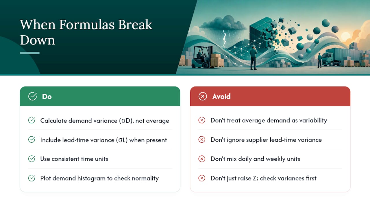
The most common mistake is using an average demand figure as if it captures variability, when it explicitly doesn’t. A SKU that sells exactly 40 units every single day and a SKU that swings between 10 and 70 units both average 40, but they need dramatically different safety stock levels. If your planning team is eyeballing “average demand times a buffer percentage” without ever calculating σD, you’re solving the wrong problem.
A second frequent error is ignoring lead-time variance entirely and using the simplified formula (SS = Z × σD × √L) on suppliers who are actually unreliable. If your supplier’s delivery window swings by three or four days regularly, dropping σL from the calculation understates your real risk, sometimes substantially.
Inconsistent time units, mixing daily demand with weekly lead time without converting, is a mechanical error that produces a confident-looking but wrong number. And failing to adjust for promotions or seasonality means your σD calculation captures noise from events that won’t repeat in the same pattern, distorting your buffer in either direction depending on when you happened to pull the data.
The statistical assumptions themselves, normality and independence, are worth checking rather than assuming. If your demand history shows a long tail of occasional huge orders (common in B2B) rather than a smooth bell curve, the normal-distribution math underlying Z-scores starts to misrepresent your actual risk. A quick visual check, plotting your demand history as a histogram, tells you in seconds whether it looks roughly bell-shaped or skewed with outliers.
Corrective steps when you spot these issues: strip out known one-time events before recalculating σD, recalculate on a rolling cadence (monthly for A items) rather than setting-and-forgetting, and shift to a Type II service-level approach or simulation for SKUs where the normal-distribution assumption clearly doesn’t hold.
Pro Tip: If a SKU has stocked out three or more times in the last two quarters despite having a calculated safety stock buffer, don’t just raise the Z-score and call it fixed. Check whether σD or σL actually reflects current reality first, since a stale variance estimate is a more common root cause than an undersized service-level target.
When to Move Beyond the Standard Formula
For most SKUs, the statistical formula covers you well. But for a subset of critical items, usually the ones with the highest stockout cost or the most erratic demand, it’s worth knowing what comes next.
Type II service level, sometimes called fill rate, measures the proportion of units demanded that get fulfilled from stock, rather than the probability of avoiding a stockout at all during a cycle (that’s Type I, which is what the standard Z-score formula targets). The math behind Type II involves what’s called the unit-loss integral, a function that relates your chosen Z-score to expected shortage quantity rather than just shortage probability. You don’t need to derive this by hand, most inventory optimization software handles it, but understanding the distinction matters when a stakeholder asks why your 95% service-level SKU still occasionally runs short: Type I and Type II answer subtly different questions.
Monte Carlo simulation earns its place when demand clearly isn’t normally distributed, when lead time varies wildly from order to order, or when the cost of getting the safety stock number wrong is high enough to justify the modeling effort. Rather than solving a closed-form equation, simulation runs thousands of randomized demand-and-lead-time scenarios based on your historical distribution and reports the safety stock level that would have prevented stockouts in, say, 98% of those simulated scenarios.
The honest signal that you’ve outgrown the classical formula isn’t complexity for its own sake, it’s when your back-tested results keep missing reality by a wide margin despite clean inputs. That’s usually a sign your demand pattern doesn’t fit the normal-distribution assumption the whole formula rests on.
Practical indicators that justify the jump: demand history with frequent zero-sales days mixed with occasional large spikes, lead times that vary by more than 50% of their average, or SKUs where a single stockout costs you a contract or a major customer relationship.
How Safety Stock Plugs Into Your Reorder Point and Ordering Policy
Safety stock isn’t a standalone number sitting on a shelf report somewhere, it’s a direct input into your reorder point, which in turn drives when your ERP or WMS actually triggers a purchase order.
ROP = E(L) × E(D) + SS
Using the earlier statistical example, expected lead-time demand of 280 units (40 daily × 7-day lead time) plus 142 units of safety stock gives a reorder point of 422 units. When on-hand inventory hits that number, your system should fire a replenishment order automatically, assuming the field is configured correctly.
Order quantity interacts with this in a specific way: if you’re using economic order quantity logic to determine how much to order each cycle, a longer interval between orders (driven by a large EOQ) means more time exposed to demand variability between reorder points, which can justify a slightly larger safety stock buffer even at the same service-level target. Shorter, more frequent order cycles reduce that exposure window and can allow a leaner buffer.
For teams operating multiple fulfillment centers, the math gets more layered. Safety stock calculated at a single national level tends to understate what you actually need once inventory is split across regional locations, because splitting demand across nodes increases the relative variability each node experiences even if aggregate national demand looks stable. A quick checklist for validating your system configuration after any safety-stock policy change:
- Confirm the ROP field in your ERP actually pulled the new SS value, not a cached old number.
- Verify time units match between your demand data and your ERP’s native demand-per-period setting.
- Cross-check that order quantity and reorder point aren’t conflicting, an EOQ that’s smaller than your safety stock buffer signals a configuration error.
- Spot-check three SKUs manually against your spreadsheet calculation before trusting the bulk upload.
- Calculate SS using the appropriate formula for the SKU tier.
- Add expected lead-time demand to get ROP.
- Load ROP and reorder quantity into the ERP’s replenishment parameters.
- Confirm the system triggers correctly on the next cycle by monitoring the first two or three reorders manually.
A Repeatable Checklist for Calculating and Maintaining Safety Stock
Running the formulas once is the easy part. Keeping them accurate as demand shifts and suppliers change is where most policies quietly go stale. Here’s a compact process to follow, informed by the kind of stepwise operational guidance APICS training materials provide for practitioners running this at scale.
- Extract data: pull 12+ months of demand history and lead-time records for each SKU from your ERP and WMS.
- Validate inputs: check for anomalies, promotions, and data gaps before calculating averages and standard deviations.
- Choose the formula: match the SKU tier (A/B/C) to the appropriate method from the framework above.
- Compute SS and ROP: run the calculation, ideally in a standardized template rather than a one-off spreadsheet.
- Upload to ERP: load the new values into the reorder point and reorder quantity fields.
- Monitor: track fill rate and stockout frequency for at least one full cycle after the change.
For the one-page master template, keep these columns: SKU ID, tier (A/B/C), E(D), σD, E(L), σL, Z, calculated SS, ROP, last recalculation date, and current fill rate. That last column matters more than people expect, since it’s your early warning system if a formula choice was wrong.
- Recalculate A items monthly, since they carry the highest revenue exposure and the most volatile demand patterns.
- Recalculate B items quarterly.
- Recalculate C items semi-annually, since the cost of staleness here is lower.
If unexpected stockouts or overstocks appear shortly after a parameter change, don’t assume the formula is broken. Check first whether the underlying σD or σL inputs were pulled from a data range that included an anomaly, that’s the more common root cause than the math itself.
What I’ve Learned Watching Safety Stock Policies Succeed and Fail
The gap between a correct formula and a working inventory policy is almost always a data problem, not a math problem. I’ve seen teams implement the full statistical formula flawlessly and still get burned, because nobody checked whether their σD calculation was quietly polluted by a three-week promotional spike from eight months earlier. The formula did exactly what it was told to do. It just wasn’t told the truth about the SKU’s real variability.
If you’re rolling out a new safety stock methodology, resist the urge to apply it catalog-wide on day one. Pick a mid-volume category, run it for one full cycle, and watch two numbers closely: fill rate and inventory days of supply. If fill rate holds steady while days of supply drops, the formula is doing its job, freeing up capital without costing you sales. If fill rate dips, your inputs need another look before you scale further.
Getting this right matters more than most planning teams initially credit it, because a miscalibrated safety stock policy doesn’t fail loudly. It fails quietly, month after month, either in the form of cash tied up in inventory nobody’s watching or in a string of near-miss stockouts that never quite get investigated as a pattern. Teams that treat safety stock as a policy to maintain, rather than a number to calculate once, tend to be the ones who catch the drift before it costs them a customer. When the scale of the rollout outpaces internal bandwidth, that’s usually when it makes sense to bring in outside support to design the tiering and get the ERP fields configured correctly from the start.
Getting Help Implementing a Safety Stock Policy Across Your Catalog
Running these formulas on a handful of SKUs in a spreadsheet is manageable on your own. Rolling out a tiered safety stock policy across a full catalog, with correct ERP parameterization, SKU segmentation, and a pilot that actually measures fill rate before you scale, is a different kind of project, and it’s exactly where 3plcowboy works with brands and 3PL providers directly.

The services map closely to what this guide walks through: designing the tiering logic for your specific catalog, configuring reorder point and safety stock fields correctly inside your ERP or WMS, and running a structured pilot with clear KPIs before committing to a catalog-wide rollout. Typical engagements focus on reducing stockout frequency on A-tier items while trimming carrying costs on the C-tier SKUs that were quietly overprotected under a one-size-fits-all policy. If your team has the formulas but not the bandwidth to implement them correctly across hundreds of SKUs, reach out to 3plcowboy to scope a pilot engagement.
Sources
- How to Calculate Safety Stock – SC Clarity