
ABC inventory analysis ranks SKUs by their annual consumption value (unit cost multiplied by annual units sold) and sorts them into three tiers. The top tier, usually 10 to 20% of SKUs drives most of your inventory value, so you count it more often, forecast it more carefully, and negotiate harder with suppliers on it. Everything downstream, from cycle-count schedules to reorder points, follows from that ranking.
TL;DR:
- The top 20% of SKUs usually account for 70 to 80% of inventory value, guiding more frequent counts and tighter forecasting for these items.
- Accurate classification relies on clean data and consistent metrics, such as cost times volume or margin contribution, with regular refreshes matching catalog dynamics.
- Classes should be aligned with operational policies, with high-value A items counted weekly, while C items may be scheduled quarterly to optimize labor and accuracy.
- Incorporating demand variability through ABC-XYZ segmentation helps tailor safety stocks and reorder points, especially for high-value, erratic demand items.
- Proper governance, including owner assignment and change logging, is essential to prevent classification drift and ensure the system’s long-term effectiveness.
Table of Contents
- What Is ABC Inventory Analysis and How Does It Relate to Pareto?
- How Do You Calculate ABC Inventory Classification?
- A Worked Example of Sorting and Classifying SKUs
- How to Perform ABC Analysis: A Step-by-Step Playbook
- What Operating Rules Should Each Class Follow?
- Best Practices and Common ABC Analysis Mistakes
- How Does ABC-XYZ Segmentation Improve Inventory Strategy?
- Using ABC Analysis to Build Cycle Counting Schedules
- When Should You Refresh ABC Classifications?
- What Operators Get Wrong About ABC Analysis
- Getting Help Implementing ABC Inventory Analysis
- Sources
- FAQ
What Is ABC Inventory Analysis and How Does It Relate to Pareto?
ABC classification inventory work rests on one observation: a small share of your catalog usually accounts for most of your dollar value. That’s the same pattern behind the Pareto principle, the 80/20 rule first applied to wealth distribution and later adopted across operations and finance. In warehousing, it shows up as a handful of SKUs, often 15 to 20% of the total, generating 70 to 80% of annual consumption value.
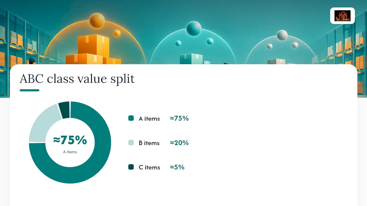
Common thresholds set A items at roughly the top 70 to 80% of cumulative value, B items at the next 15 to 25%, and C items at the remainder, according to CIPS guidance on ABC classification. Those numbers are starting points, not law. A catalog with a few dominant products might push the A threshold to 85%, while a long-tail catalog with thousands of low-volume SKUs often works better with A set closer to 60 to 70%, per InventoryQuick’s threshold guidance.
Ranking by cost times volume isn’t the only option. Depending on what you’re optimizing for, consider:
- Margin contribution when profitability matters more than raw volume, especially in categories with wide markup variance.
- Pick frequency when your bottleneck is labor hours, not capital tied up in stock.
- Consumption value (the default) when the goal is prioritizing counting, forecasting, and supplier attention.
Pick one primary metric and stay consistent. Mixing metrics between refresh cycles is how classifications drift and trust in the system erodes.
How Do You Calculate ABC Inventory Classification?
The math behind an abc classification method is simple arithmetic run across your full SKU list. The hard part is getting clean inputs. Before you calculate anything, pull these fields for every active SKU:
- SKU identifier and description, deduplicated so no item shows up under two codes.
- Unit of measure (UOM), standardized so you’re not multiplying cases by one SKU and eaches by another.
- Unit cost, ideally landed cost including freight, not just PO price.
- Trailing 12-month unit demand, pulled from shipped or consumed units, not forecast.
- Flag for new or discontinued items, since a 3-month-old SKU with a demand spike can skew results if treated like a mature item.
Once the data’s clean, the formula sequence is:
| Step | Formula (spreadsheet syntax) |
|---|---|
| Annual consumption value | =UnitCost * AnnualUnits |
| % of total value | =ACV / SUM(ACV_range) |
| Cumulative % | =SUM($ACV$1:ACV_current) / SUM(ACV_range) |
| Class assignment | =IF(CumulativePct<=0.7,"A",IF(CumulativePct<=0.9,"B","C")) |
Sort descending by annual consumption value before running the cumulative percent formula. That sort order is what makes the cumulative math meaningful. For a tie-break, when two SKUs land at the exact same value, the Cleverence guide to the ABC method recommends breaking ties by criticality or lead time risk rather than alphabetically.
On the rolling window, a trailing 12-month period works for most catalogs. Seasonal or fast-moving categories sometimes benefit from a 6-month window refreshed quarterly, while capital equipment or slow movers are better served by a 24 to 36-month window that smooths out lumpy, infrequent orders.

A Worked Example of Sorting and Classifying SKUs
Here’s a 10-SKU example that shows the full sequence, from raw inputs to final class.
This is exactly the straddle case the InventoryQuick playbook flags, and the safer move is to round it up to A rather than leave it as a B, since underprotecting a revenue-significant item costs more than an extra count cycle.
That single reclassification changes real policy:
- SKU-330 moves from monthly cycle counts to weekly, and its reorder point gets recalculated with a tighter safety margin.
- SKU-156 stays a C item, meaning it gets a quarterly count, a simple min/max reorder trigger, and no dedicated forecasting attention.
How to Perform ABC Analysis: A Step-by-Step Playbook
Running an abc inventory strategy for the first time is less about the math and more about sequencing the work so the output survives contact with your ERP.
- Extract and clean the SKU master. Pull unit cost, UOM, and 12-month demand from your ERP or WMS. Reconcile duplicate SKU codes and flag anything discontinued in the last 90 days so it doesn’t distort rankings.
- Compute usage value and assign classes. Run the formulas above in a spreadsheet or your inventory optimization software, sort descending, and apply the cumulative-percent cutoffs.
- Translate classes into policies. For each class, define count cadence, reorder logic, and a named owner. Without an owner, the classification becomes a report nobody acts on.
- Pilot before you roll out. Test the full cycle, classify, assign policy, and count, on one distribution center or one product family for 30 to 60 days before pushing it company-wide.
- Document and control changes. Log every class change with a timestamp and reason. If more than roughly 10 to 15% of SKUs shift class in a single refresh, investigate before accepting the new classification. That’s usually a data problem, not a real demand shift.
The Sage guide to ABC analysis frames this as a five-step cycle tied to forecasting software, which lines up with what actually works in practice: the classification step is the easy part, and the governance around it is where programs succeed or quietly die.
Pro Tip: Run your pilot on the product family with the messiest demand pattern, not the cleanest one. If ABC holds up under your worst data, it’ll hold up everywhere else.
Piloting on a single DC also gives you a controlled place to test how classification changes ripple into inventory optimization workflows before you touch slotting or labor planning company-wide.
What Operating Rules Should Each Class Follow?
Classes only matter once they change what happens on the floor. Here’s how cadence and policy typically split out:
- A items: weekly or biweekly cycle counts, tight reorder points, safety stock tuned against actual demand variability, and placement in prime pick locations closest to packing stations.
- B items: monthly counts, standard reorder logic, moderate safety stock, and mid-tier slotting.
- C items: quarterly counts, simple min/max triggers, and minimal forecasting attention beyond flagging dead stock.
Vary those defaults when the situation calls for it. A items with long supplier lead times may need biweekly counts and elevated safety stock, while stable C items with reliable local suppliers can sometimes stretch to semiannual counts without risk.
Assign a named owner to A-class SKUs specifically. That person tracks fill rate, turns, and forecast accuracy for their assigned items and flags anomalies before they become stockouts. B and C items can be managed at the category level rather than SKU by SKU, since the labor cost of individual attention doesn’t pay off at that value tier.
Set class-level KPIs rather than one blanket target. A reasonable structure tracks fill rate and forecast accuracy for A items, turns and carrying cost for B items, and dead-stock percentage for C items, since chasing a single company-wide service-level number tends to overinvest in low-value SKUs and underprotect the ones that matter.
Best Practices and Common ABC Analysis Mistakes
Criticality should override pure value ranking for a specific subset of items: parts that halt a production line, components tied to regulatory compliance, or single-source items with long lead times. Promote those to A treatment regardless of what the cumulative percentage says. A $2 gasket that stops an assembly line is not a C item just because its annual consumption value is low.
Master-data governance is what separates a program that lasts from one that decays after a quarter. Assign a data owner, set a fixed refresh cadence, and keep a change log that records what moved classes and why, as the master-data governance research on ABC-XYZ systems emphasizes.
Three mistakes show up constantly in abc inventory segmentation projects:
- Ranking by unit price instead of usage value. A $500 item that sells twice a year is not more important than a $5 item that sells 50,000 times.
- Set-and-forget classification. Demand shifts, and a class assigned in January can be wrong by July.
- Ignoring demand variability entirely. Two A items with identical annual value can need completely different safety-stock strategies if one is steady and the other spikes unpredictably.
Pro Tip: Keep a running exceptions list for criticality overrides separate from your main ABC table. It makes audits faster and stops the override logic from getting buried in a formula nobody remembers writing.
How Does ABC-XYZ Segmentation Improve Inventory Strategy?
Layering variability on top of value is what turns abc xyz segmentation into a genuinely useful planning tool. XYZ bands classify demand predictability: X items have stable, easy-to-forecast demand, Y items show moderate seasonal or trend variation, and Z items are erratic with little pattern.
Cross ABC with XYZ and you get nine cells, each with a different playbook:
- A-X items (high value, stable demand): tight reorder points, minimal safety stock, ideal candidates for vendor-managed inventory.
- A-Z items (high value, erratic demand): the riskiest cell. These need higher safety-stock buffers, flexible supplier terms, and sometimes consignment arrangements to avoid tying up cash on units that might not move on schedule.
- C-Z items: often not worth active management at all beyond periodic dead-stock review.
The research is clear that abc xyz analysis only delivers those gains when paired with disciplined master-data governance and a periodic refresh cycle. Without that discipline, the nine-cell matrix becomes stale within a couple of quarters and the extra complexity stops paying for itself.
Using ABC Analysis to Build Cycle Counting Schedules
A cycle-count schedule built on ABC classes replaces the old approach of counting everything once a year during a shutdown. Instead:
- A items get counted weekly or biweekly, generating count sheets pulled directly from the WMS and filtered by class.
- B items get counted monthly, often batched by location zone to minimize walking time.
- C items get counted quarterly, frequently as part of a broader zone sweep rather than a standalone event.
Run those count sheets on handheld or mobile WMS devices so discrepancies get flagged and investigated same-day instead of surfacing weeks later during a full physical count.
Track count accuracy by class separately, not as one blended number. A program that hits 99% accuracy on C items but 90% on A items has a real problem masked by the average. Watch pick and putaway error rates alongside fill rate and working-capital metrics to see whether the classification is actually reducing risk where it counts most. One operation moved from 61% to over 98% cycle-count accuracy across 450,000-plus SKUs by tightening exactly this kind of class-based count discipline. For more on rebuilding count accuracy without new technology, see how operators fix inventory accuracy.
When Should You Refresh ABC Classifications?
Refresh cadence depends on how fast your catalog moves. Fast-turning categories, like fashion or seasonal CPG, need a monthly review. Stable, slow-moving catalogs, industrial parts or raw materials, can run on a quarterly cycle without losing accuracy.
Put a change-control limit on every refresh.
Watch these signals to confirm the program is working rather than drifting:
- Service level by class, tracked separately for A, B, and C.
- Expedite frequency, which should trend down for A items as forecasting improves.
- Inventory turns and weeks of supply by class.
- Working capital tied up in each tier, since a shrinking share locked in C items is a sign the classification is doing its job.
What Operators Get Wrong About ABC Analysis
Most ABC rollouts fail from neglect, not bad math. Teams run the classification once, print the report, and never touch it again. The formula takes an afternoon. The governance, the owner assignments, the refresh discipline, is what takes real work and what most programs skip.
The checklist that actually holds up: clean the SKU master before you calculate anything, assign a named owner per class, pilot on one DC or product family, and put change-control limits on every refresh. Skip any one of those four and the classification degrades within two quarters. The math never changed. The discipline around it did.
— Michael
Getting Help Implementing ABC Inventory Analysis
Running the calculation is straightforward. Making it stick across a full SKU catalog, multiple warehouses, and a team that has to actually change how it counts and reorders is where most in-house efforts stall. 3plcowboy brings 17-plus years of hands-on operating experience, not consulting theory, to exactly that gap: turning a spreadsheet classification into governed, repeatable policy that survives past the first quarter.

If your team is weighing whether to build this internally or bring in outside help, the honest answer depends on scale. A single-location operation with a stable catalog can often run ABC in-house with the playbook above. A multi-DC network with thousands of SKUs, seasonal swings, and a history of classification drift usually benefits from an outside set of eyes that has rebuilt these systems before. 3plcowboy’s 3PL Operations Advisory works directly on accuracy improvements, working-capital reduction, and building the governance structure that keeps a classification system honest quarter after quarter. Review the full range of services, including fulfillment cost benchmarking and network design, on the services page, and start a conversation about what your catalog actually needs.
Sources
For a spreadsheet template with pre-built thresholds and a worked example, the InventoryQuick worksheet and playbook covers per-class cadences in practical detail. For the governance research behind pairing ABC with variability analysis, see the MDPI study on ABC-XYZ master-data governance. For formula-level detail and best-practice framing, the Cleverence guide to the ABC method is a solid reference, and CIPS’s overview of ABC classification is useful for the procurement side of threshold-setting.
- ABC Analysis for Inventory: Thresholds, Worksheet & Playbook (InventoryQuick)
- ABC classification & ABC method | CIPS
FAQ
What Is ABC Analysis in Inventory Management?
ABC analysis is a method for ranking SKUs by their contribution to annual consumption value and sorting them into three tiers: A (highest value), B (moderate), and C (lowest). A items typically make up the top 70 to 80% of cumulative value despite being a small share of total SKUs, according to CIPS.
How Do You Calculate ABC Inventory Classification?
Multiply each SKU’s unit cost by its trailing 12-month unit demand to get annual consumption value, then sort descending and calculate cumulative percentage of total value.
What Are Some Real Examples of ABC Analysis?
That kind of concentration is common enough that many practitioners plan around it as a default assumption.
What Is the Difference Between ABC Analysis and EOQ?
ABC analysis segments SKUs by value to prioritize management attention and counting frequency. Economic order quantity (EOQ) is a separate formula that calculates the ideal order size for a single SKU by balancing ordering costs against holding costs. Teams often run ABC first to decide which SKUs deserve the more detailed EOQ calculation.
Does 3plcowboy Help Implement ABC Inventory Analysis?
Yes. 3plcowboy’s 3PL Operations Advisory and broader services cover operational improvement work, including inventory classification governance and accuracy programs. Pricing is available on request through the site.